Studying the Behaviour of Projection Pursuit Indices

A practical tour of the five most important functions in spinebil for finding, validating, and understanding projection pursuit indices.

Overview

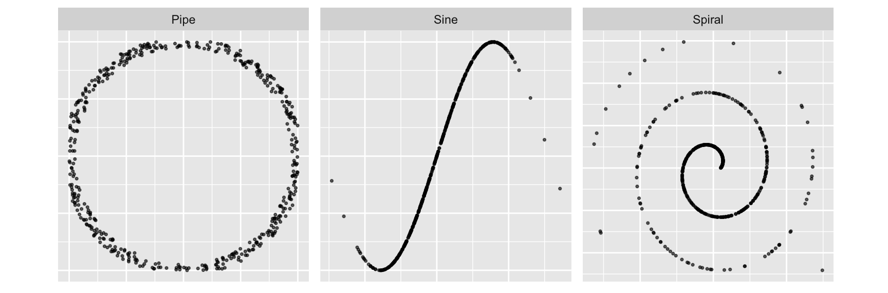
In this vignette we introduce three example datasets; spiral, a sine, and a pipe dataset and then evaluate five key characteristics of projection pursuit indices (PPIs): smoothness, squintability, flexibility, rotation invariance and speed.

We will generate the datasets first, then walk through one section per characteristic with the functions provided in spinebil.

Data Generators

pipe_data(n, p, t); a pipe (circular ring) structure.
sin_data(n, p, f); a sine relationship.
spiral_data(n, p); an archimedean spiral.

n <- 500
p <- 4
lst <- list(
  Pipe   = spinebil::pipe_data(n, p),
  Sine   = spinebil::sin_data(n, p, 1),
  Spiral = spinebil::spiral_data(n, p)
)

df_all <- do.call(rbind, lapply(names(lst), function(lbl) {
  d <- lst[[lbl]]
  data.frame(x = d[[p - 1]], y = d[[p]], structure = lbl)
}))

ggplot2::ggplot(df_all, ggplot2::aes(x, y)) +
  ggplot2::geom_point(alpha = 0.6, size = 0.6) +
  ggplot2::facet_wrap(~ structure, nrow = 1, scales="free") +
  ggplot2::theme(
    aspect.ratio = 1,
    axis.text  = ggplot2::element_blank(),
    axis.ticks = ggplot2::element_blank(),
    axis.title = ggplot2::element_blank()
  )

Now we employ these patterns to evaluate key characteristics of PPIs.

1) `compare_smoothing()`

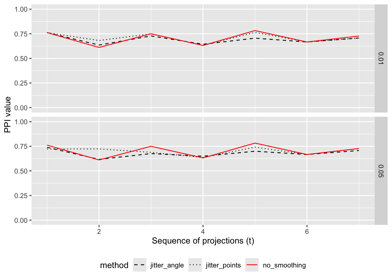
Projection pursuit indices evaluated along a tour path can be spiky due to small numerical changes in the projection or to point-level noise. compare_smoothing() provides a principled way to smooth these traces by averaging the index over local perturbations, and to compare different smoothing strategies side-by-side.

It supports two kinds of perturbations:

jitter_angle: randomly jitter the projection plane by a small angle alpha via geodesic moves, then recompute the index.
jitter_points: randomly jitter the projected points by a small amount (using base::jitter()), then recompute the index.
no_smoothing: the original index with no perturbation.

Averaging across multiple perturbations reduces high-frequency noise and reveals the underlying trend of the index along the tour.

Function Usage

compare_smoothing(
  d,         # data matrix (n x p)
  tPath,     # interpolated tour path: list of projection bases (p x 2)
  idx,       # index function
  alphaV = c(0.01, 0.05, 0.1),  jitter amounts to compare (for jittering angle or points)
  n = 10     # number of evaluations entering mean value calculation
)

Inputs

d, numeric data matrix with p columns. It will be projected as d %*% basis for each basis in tPath.
tPath, list of (p × 2) projection bases. Typically built from a tour history using tourr::save_history() and tourr::interpolate().
idx, index function accepting a two-column matrix and returning a single numeric value (e.g., scag_index("stringy")).
alphaV, numeric vector of jitter magnitudes to compare.
n, number of evaluations entering mean value calculation (larger n → smoother, slower).

Example Usage

d <- as.matrix(spinebil::spiral_data(30,4))
tPath <- tourr::save_history(d, max_bases=2)
tPath <- as.list(tourr::interpolate(tPath, 0.3))
idx <- spinebil::scag_index("stringy")
compS <- spinebil::compare_smoothing(d, tPath, idx, alphaV = c(0.01, 0.05), n=2)
spinebil::plot_smoothing_comparison(compS, lPos = "bottom")

Interpretation

no_smoothing (red, solid): the raw index trace along the tour. Spiky traces indicate high sensitivity to tiny projection changes.
jitter_angle (black, dashed): averaging over nearby projection angles. Smooths out high‑frequency variability caused by small plane movements; preserves structure amplitude better when index is robust to minor orientation shifts.
jitter_points (black, dotted): averaging over point noise. Strong smoothing when the index is sensitive to local point perturbations.

Return value

A tibble with columns:

index_mean, mean index value at each frame (includes the original, unjittered value).
t, integer frame index along the tour path.
method, one of "jitter_angle", "jitter_points", "no_smoothing".
alpha, jitter magnitude used for that row.

2) `squint_angle_estimate()`

From how far away (in projection space) does the pattern become visible under a chosen index?

squint_angle_estimate(), produces a distribution of squint angles by repeatedly walking from random 2‑D planes toward an assumed optimal plane (the best view of a structure) and recording the first point along each path where a user‑chosen index function exceeds a visibility cutoff.

Interpretation:

Larger squint angles ⇒ easier to see (the index crosses the cutoff while still far from the optimal plane).
Smaller squint angles ⇒ harder to see (the index only crosses when we are very close to the optimal plane).

Function usage

squint_angle_estimate(
  data,            # numeric matrix/data frame (n x p)
  indexF,          # function: (n x 2) -> numeric scalar
  cutoff,          # numeric threshold for 'visible'
  structure_plane,  # 2-D basis (p x 2) representing the optimal view
  n = 100,         # number of random starts
  step_size = 0.01  # interpolation step along the tour path
)

Example Usage

data <- as.matrix(spinebil::spiral_data(50, 4))
indexF <- spinebil::scag_index("stringy")
cutoff <- 0.7
structure_plane <- spinebil::basis_matrix(3,4,4)
spinebil::squint_angle_estimate(data, indexF, cutoff, structure_plane, n=10)
#>  [1] 0.9539643 1.4172710 1.0504801 1.2003548 1.4036393 1.4239164 1.6173852
#>  [8] 1.0675589 1.3543386 0.9873721

Inputs

`indexF` (what kind of structure?)

Choose an index that matches the pattern you care about. With scagnostics-style indices, for example:

indexF <- scag_index("stringy")   # sine-wave/spiral-like
indexF <- scag_index("skinny")  # elongated patterns

`cutoff` (when do we call it visible?)

Set this data‑driven so results are comparable across datasets and indices.

Preferred: 95th–99th percentile of the index computed on random projections (a null where no specific structure is targeted).
You can use index_noise_threshold() to estimate this cutoff automatically.

`structure_plane` (where is the best view?)

If you know the two variables that define the structure, construct the basis directly. Otherwise, run a guided tour to maximize the index and use the best basis it returns.

`n` and `step_size`

n = 100 typically yields a stable distribution for summaries and plots.
step_size = 0.01 is a good accuracy/speed trade‑off. If the threshold crossing looks coarse (the index jumps over the cutoff), try 0.005. If runtime is an issue, use something larger (e.g., 0.02).

Return value

squint_angle_estimate() returns a numeric vector of length n containing the squint-angle estimates under the specified index and cutoff.

3) `get_trace()`

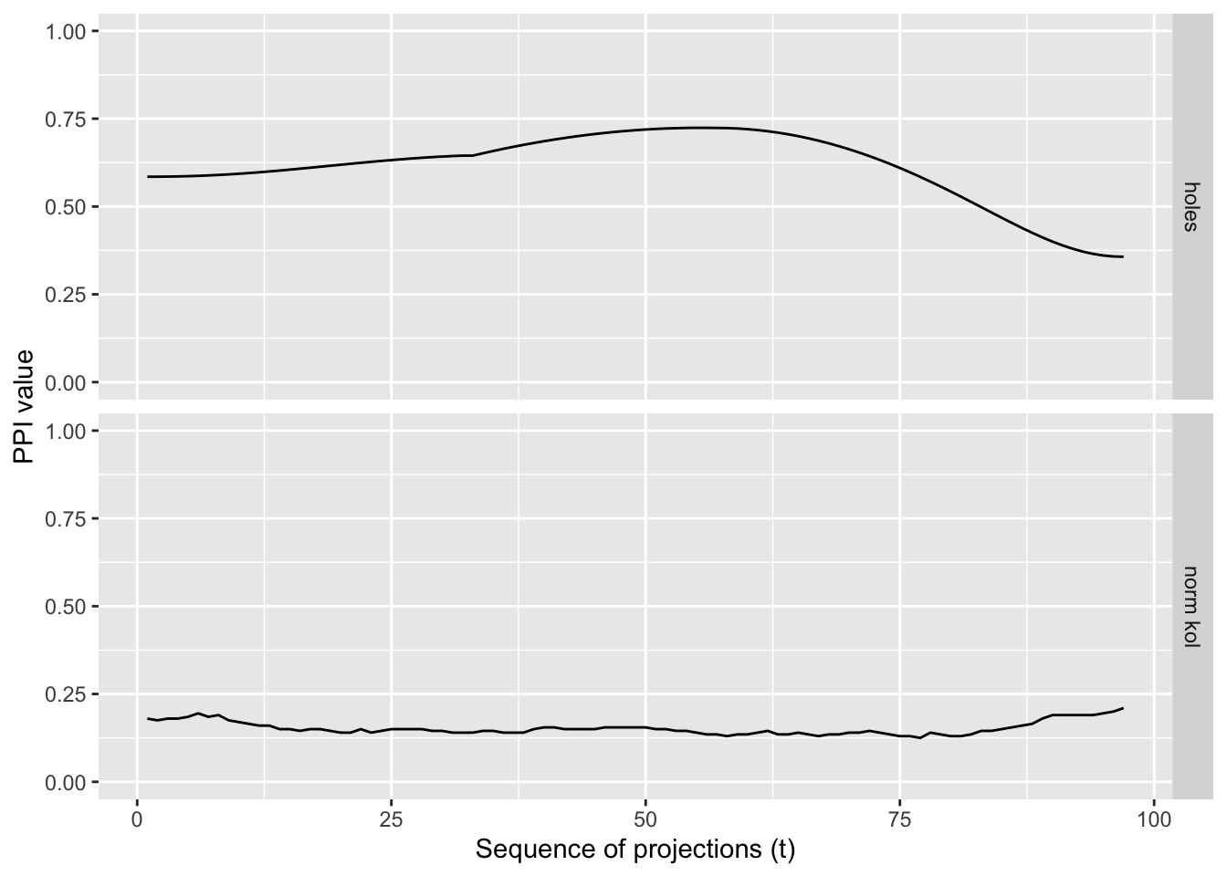
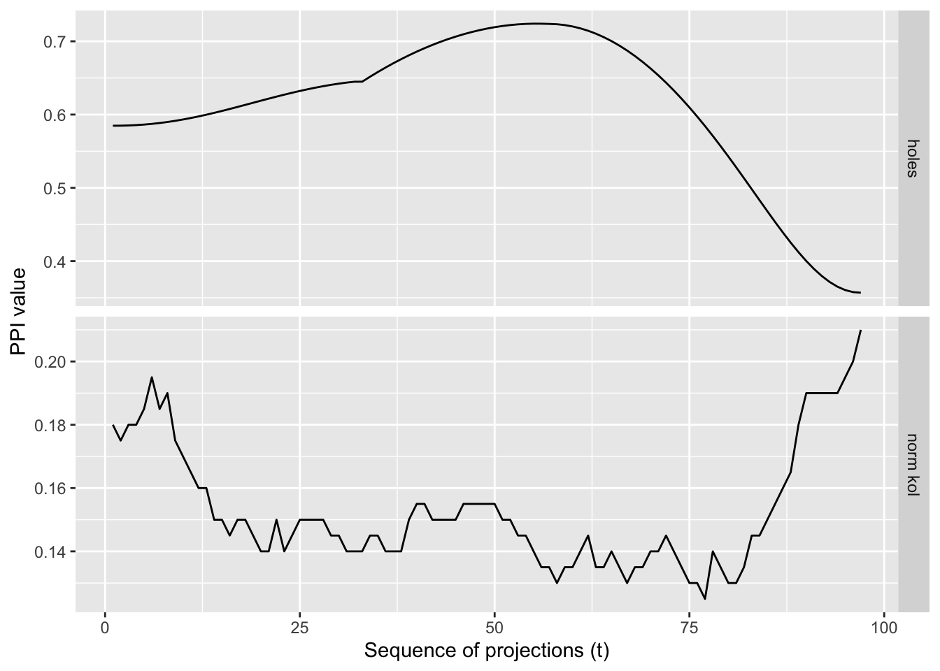
get_trace() evaluates one or more projection pursuit indices along an interpolated, planned tour path and returns their values at each frame. Plotting these traces reveals whether an index varies smoothly with small changes in the projection (desirable), or exhibits spikes (potentially unstable, overly sensitive, or under‑smoothed).

A smooth trace indicates that small rotations of the view produce small changes in the index,an important property for guided tours and optimisation.

In combination with plot_trace(), you can quickly diagnose index behaviour across a path connecting user‑specified views.

Function Usage

get_trace(
  d,           # data: matrix/data frame (n x p)
  m,           # list of projection matrices for the planned tour
  index_list,   # list of index functions to calculate for each entry -> numeric
  index_labels  # character vector of labels for the indices
)

Inputs

d; numeric data with p columns.
m; list of (p × 2) projection matrices for the planned tour.
index_list; list of functions that take a two‑column matrix and return a numeric scalar (e.g., tourr::holes(), tourr::cmass(), or scag_index("stringy")).
index_labels; character vector of the same length and order as index_list; used as column names in the output.

Example Usage

d <- as.matrix(spinebil::spiral_data(100, 4))
m <- list(spinebil::basis_matrix(1,2,4), spinebil::basis_matrix(3,4,4))
index_list <- list(tourr::holes(), tourr::norm_kol(100))
index_labels <- c("holes", "norm kol")
trace <- spinebil::get_trace(d, m, index_list, index_labels)
spinebil::plot_trace(trace)

spinebil::plot_trace(trace, rescY = FALSE)

Return value

A numeric matrix with length(index_labels) + 1 columns and as many rows as interpolation frames. Columns are the index values (named by index_labels) and t (the frame index).

4) `profile_rotation()`

Does the index value stay the same when the 2‑D data are rotated?

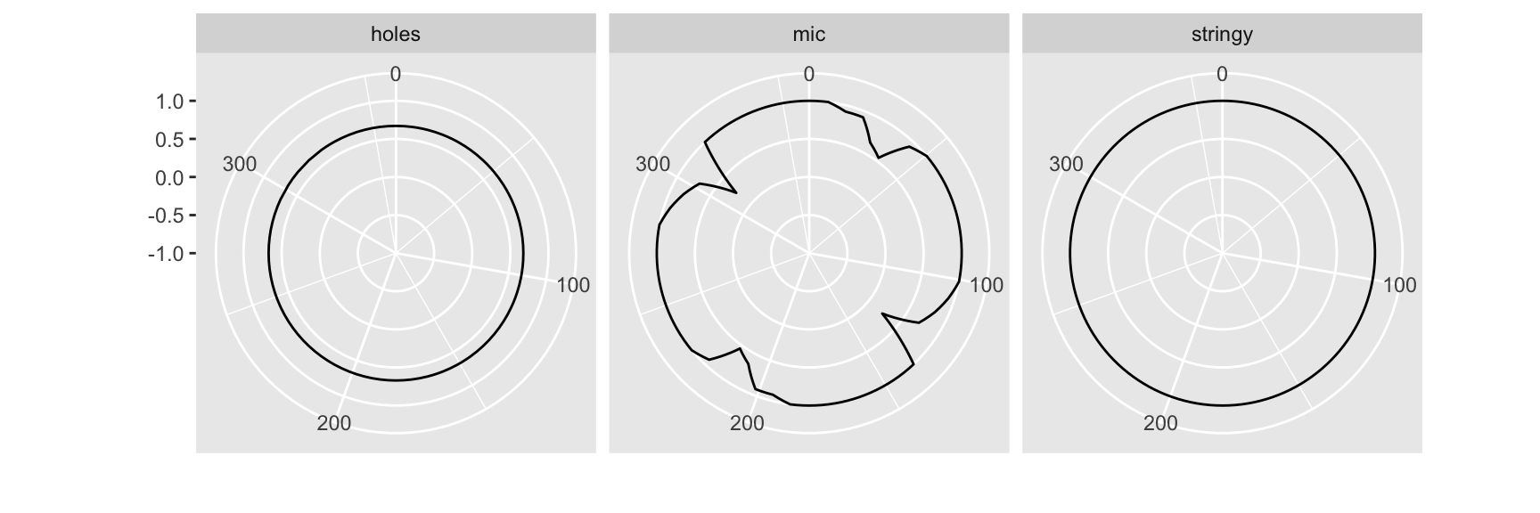
profile_rotation() tests rotation invariance of one or more 2-D projection indices.

Interpretation

Flat profile → rotation invariant.
Oscillating profile → orientation dependence.

Function Usage

profile_rotation(
  d,            # 2-column numeric matrix (the data to rotate)
  index_list,    # list of functions: (n x 2) -> numeric
  index_labels,  # character labels for columns
  n = 200       # number of rotation steps across [0, 2*pi]
)

Inputs

d: numeric matrix with 2 columns; the 2-D data to be rotated.
index_list: list of functions, each taking an $(n \times 2)$ numeric matrix and returning a single numeric index value. Examples: list(tourr::holes(), scag_index("stringy"), mine_indexE("MIC")).
index_labels: character vector of labels (one per index in index_list) used as column names in the result.
n (default = 200): integer number of rotation steps.

Example Usage

d <- as.matrix(spinebil::sin_data(30, 2))
index_list <- list(tourr::holes(), spinebil::scag_index("stringy"), spinebil::mine_indexE("MIC"))
index_labels <- c("holes", "stringy", "mic")
pRot <- spinebil::profile_rotation(d, index_list, index_labels, n = 50)
spinebil::plot_rotation(pRot)

Interpretation

Perfect circle (constant radius) → rotation invariant.
Deformed/flower-like shape → orientation dependence.

Return value

A numeric matrix with n + 1 rows and length(index_labels) + 1 columns:

One column per index (named by index_labels) containing the index values at each angle.
An additional column alpha giving the corresponding angles in radians.

5) `time_sequence()`

The cost of evaluating a projection pursuit index can vary with both the data distribution and the projection. time_sequence() times the index on a sequence of projection bases and returns a simple table you can plot or summarise.

Function Usage

time_sequence(
  d,      # numeric data matrix (n x p)
  t,      # list of projection matrices (each p x 2); e.g., an interpolated tour path
  idx,    # index function: (n x 2) -> numeric
  pmax    # maximum number of projections to evaluate (cut t if longer than pmax)
)

Inputs

d: numeric matrix of size $n \times p$ .
t: list of (p × 2) projection bases (e.g., from tourr::basis_random() or an interpolated tour history).
idx: index function mapping a two-column matrix to a single numeric value (e.g., scag_index("stringy")).
pmax: integer limit; evaluation stops after pmax projections even if t is longer.

Example Usage

d <- as.matrix(spinebil::spiral_data(500, 4))
t <- purrr::map(1:10, ~ tourr::basis_random(4))
idx <- spinebil::scag_index("stringy")
spinebil::time_sequence(d, t, idx, 10)
#>        t  i
#> 1  0.045  1
#> 2  0.050  2
#> 3  0.044  3
#> 4  0.048  4
#> 5  0.053  5
#> 6  0.048  6
#> 7  0.044  7
#> 8  0.048  8
#> 9  0.047  9
#> 10 0.048 10

Return value

A data frame with two columns:

t: elapsed time in seconds for the index evaluation at that projection.
i: the sequence index (1, 2, …) of the projection in t.

Overview

Data Generators

1) compare_smoothing()

Function Usage

Inputs

Example Usage

Interpretation

Return value

2) squint_angle_estimate()

Function usage

Example Usage

Inputs

indexF (what kind of structure?)

cutoff (when do we call it visible?)

structure_plane (where is the best view?)

n and step_size

Return value

3) get_trace()

Function Usage

Inputs

Example Usage

Return value

4) profile_rotation()

Function Usage

Inputs

Example Usage

Interpretation

Return value

5) time_sequence()

Function Usage

Inputs

Example Usage

Return value

1) `compare_smoothing()`

2) `squint_angle_estimate()`

`indexF` (what kind of structure?)

`cutoff` (when do we call it visible?)

`structure_plane` (where is the best view?)

`n` and `step_size`

3) `get_trace()`

4) `profile_rotation()`

5) `time_sequence()`