More Diagnostics for Projection Pursuit Indices

This vignette is a guide to diagnosing Projection Pursuit Indices in high-dimensional exploratory analysis. We examine how it behaves under different conditions. The goal is to help you decide which index to use, how to tune it, and how to trust its signals.

Overview

This vignette presents a workflow built around these functions: data_gen(), noise_gen(), ppi_mean(), ppi_scale(), ppi_noise_threshold() and ppi_samplesize_effect()

Packages

library(tidyverse)
library(spinebil)
library(tourr)

1) Generating Synthetic Structures and Noise

data_gen(); generate structured 2D point sets (e.g., sine, circle, cluster) or orthogonal polynomial features for benchmarking/visualisation.
- Structures (type like "sine", "circle", …) return a tibble with columns x, y, and structure.
- Polynomial (type = "polynomial") returns an n × degree matrix of orthogonal polynomial basis vectors on [0,1].
noise_gen(); generates a numeric vector of noise values (as a tibble with value and type) from distributions such as: "gaussian", "uniform", "lognormal", "t_distributed", "cauchy", "beta_noise", "exponential", "microstructure".

We’ll preview available structures, create simple polynomial features, sample a few noise types, and combine structure + noise.

Function usage

data_gen(type = "all", n = 500, degree = NULL, seed = NULL)

type: "linear", "sine", "circle", "cluster", "snake", "outliers", "sparse", "clumpy", "skewed", "striated", "concave", "monotonic", "doughnut", "all", or "polynomial".
n: number of points/samples.
degree: only for "polynomial"; number of basis columns.
seed: optional seed for reproducibility.

noise_gen(n = 500, type = "gaussian", level = 0.1, seed = NULL)

n: number of noise samples.
type: distribution name ( "gaussian", "uniform", "lognormal", "t_distributed", "cauchy", "beta_noise", "exponential", "microstructure").
level: scale/strength of noise.
seed: optional seed.

Example usage

# One structure
df_sine <- data_gen("sine", n = 400, seed = 1)

# Multiple structures at once
df_all  <- data_gen("all",  n = 400, seed = 1)

Preview all structures

ggplot(df_all, aes(x, y)) +
  geom_point(alpha = 0.6, size = 0.6) +
  facet_wrap(~ structure, scales = "free") +
  labs(title = "Synthetic 2D Structures from data_gen()",
       subtitle = "Each panel generated with n = 400")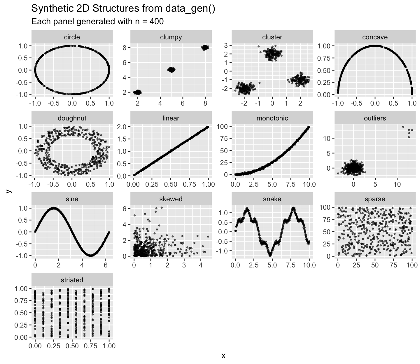

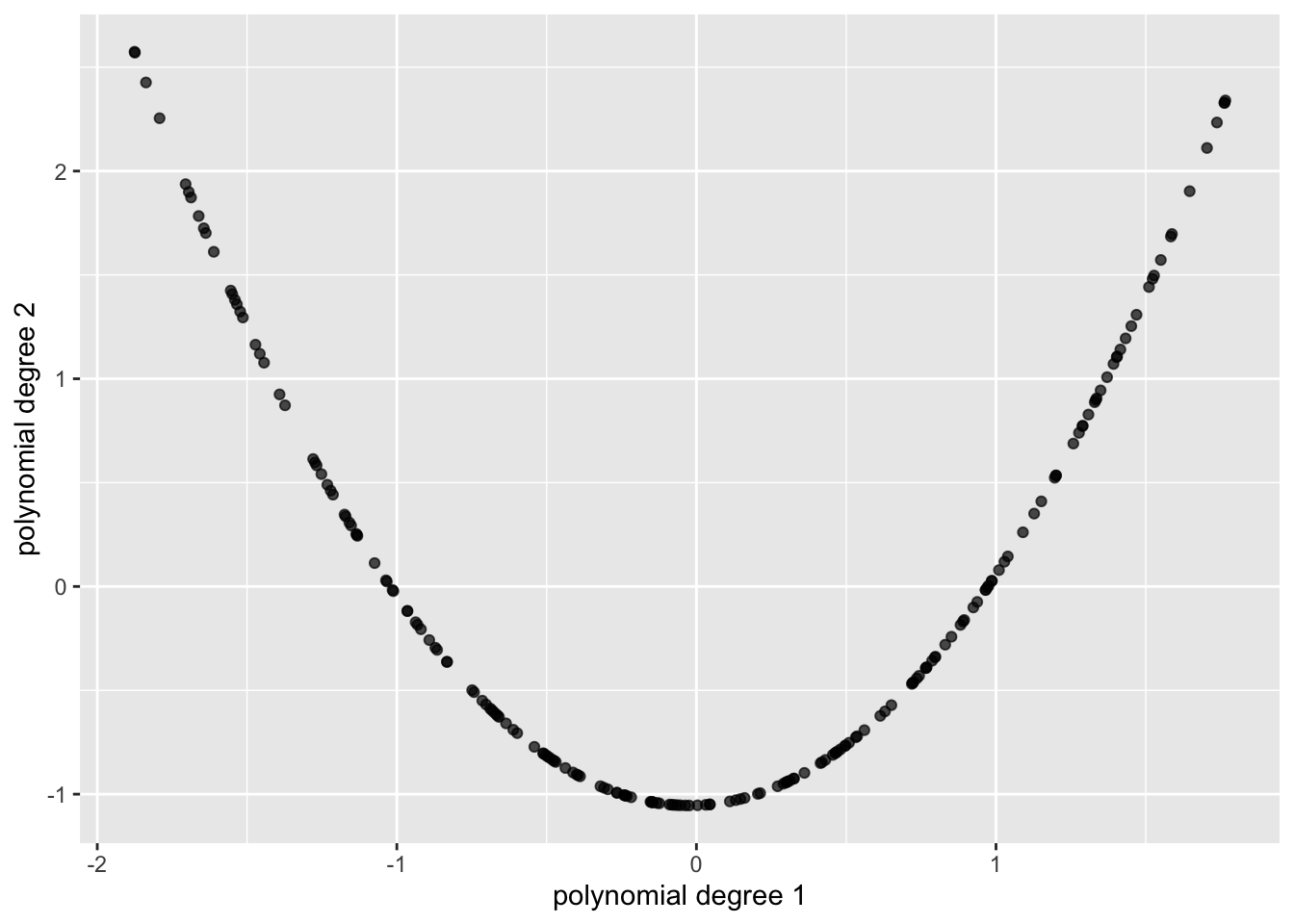
Polynomial features (`type = "polynomial"`)

# Generate a 4-degree orthogonal polynomial basis
dPoly <- data_gen("polynomial", n = 200, degree = 4, seed = 1)

ggplot(dPoly, aes(x = dPoly[,1] , y = dPoly[,2])) +
  geom_point(alpha = 0.7) + 
  xlab("polynomial degree 1") +
  ylab("polynomial degree 2")

`noise_gen()`: noise distributions

eps_g <- noise_gen(n = 500, type = "gaussian",   level = 0.06, seed = 340)
eps_t <- noise_gen(n = 500, type = "t_distributed", level = 0.15, seed = 341)
eps_cau <- noise_gen(n = 500, type = "cauchy",     level = 0.04, seed = 342)

Combining structure + noise

As a simple example, let’s take a clean sine wave and add Gaussian noise to y.

set.seed(345)
n <- 500
sine_clean <- data_gen("sine", n = n) |> mutate(y = sin(x)) 

# Noise to add on y
eps <- noise_gen(n = n, type = "gaussian", level = 0.06, seed = 123)$value
sine_noisy <- sine_clean |> mutate(y = y + eps)

bind_rows(
  sine_clean  |> mutate(which = "clean"),
  sine_noisy  |> mutate(which = "noisy (gaussian, level = 0.06)")
) |>
  ggplot(aes(x, y, color = which)) +
  geom_point(alpha = 0.6, size = 0.6) +
  labs(title = "Sine Structure with and without Added Noise",
       color = NULL)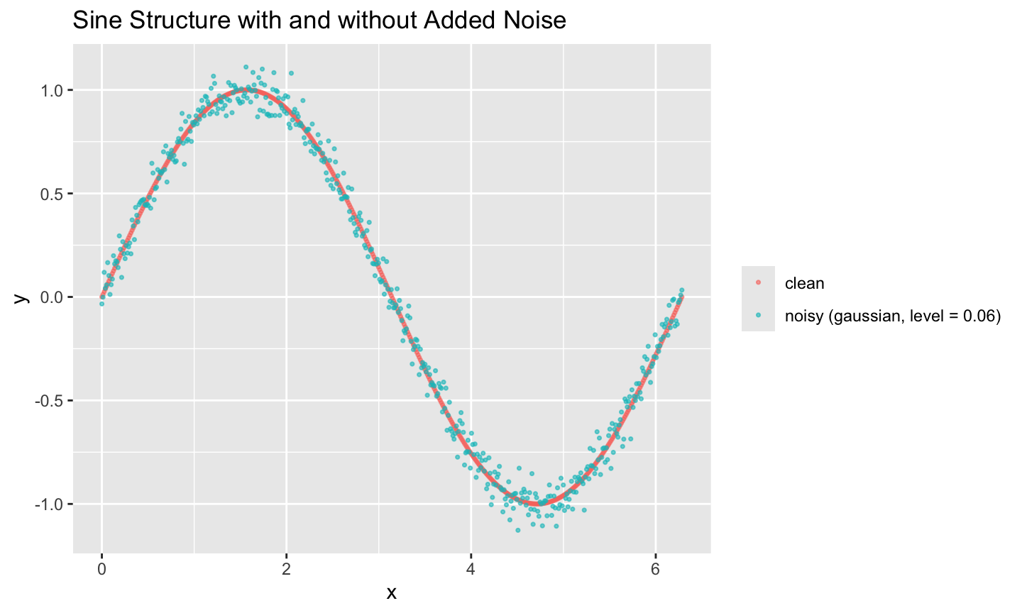

Return value

data_gen("polynomial", ...) returns an n × degree matrix.
data_gen(<other type>, ...) return a tibble with columns x, y, and structure.
noise_gen(...) returns a tibble with columns value (numeric) and type (factor/character).

2) Finding Projection Pursuit Index Mean

ppi_mean() simulates and summarizes a projection pursuit index (PPI) over all 2D variable pairs in a dataset. For each pair, it repeats the index evaluation n_sim times (sampling n_obs observations each time) and returns the mean index per pair.

Function usage

res <- ppi_mean(
  data,        # data frame with ≥ 2 numeric columns
  index_fun,   # function taking n×2 matrix and returning a numeric value
  n_sim = 100,
  n_obs = 300
)

Example Usage

data <- as.data.frame(data_gen(type = "polynomial", degree = 2))
res  <- ppi_mean(data, scagIndex("stringy"), n_sim = 5)
res
#> # A tibble: 1 × 3
#>   var_i var_j mean_index
#>   <chr> <chr>      <dbl>
#> 1 1     2              1

Return value

A tibble with one row per variable pair:

var_i, var_j; names of the variables forming the pair.
mean_index; the mean of the index across n_sim simulations for that pair.

3) Comparing Index Scale on Structured vs. Noisy Data

ppi_scale() runs simulations to compare a projection pursuit index (PPI) on:

Structured dataset (your input), and
Pure Gaussian noise (same sample size).

For every pair of variables and across many simulations, it records the index values for both cases so you can see the scale and separation of the index between structure and noise.

Function Usage

ppi_scale(
  data,        
  index_fun, 
  n_sim = 100,
  n_obs = 500,
  seed = NULL
)

Inputs:

data — data frame/tibble/matrix; (>= 2 numeric columns).
index_fun — function: takes a 2-column matrix and returns a numeric scalar (e.g., scagIndex("stringy")).
n_sim — number of simulations.
n_obs — number of observations.
seed — optional seed for reproducibility.

Example usage

Let’s evaluate the stringy index from the cassowaryr package to see how the scale change for pure noise and structure.

res <- ppi_scale(data_gen("polynomial", degree = 3), scagIndex("stringy"), n_sim = 3)

head(res)
#> # A tibble: 6 × 6
#>   simulation var_i var_j var_pair sigma index
#>        <int> <chr> <chr> <chr>    <dbl> <dbl>
#> 1          1 1     2     1-2          0 1    
#> 2          1 1     2     1-2          1 0.732
#> 3          1 1     3     1-3          0 1    
#> 4          1 1     3     1-3          1 0.783
#> 5          1 2     3     2-3          0 0.996
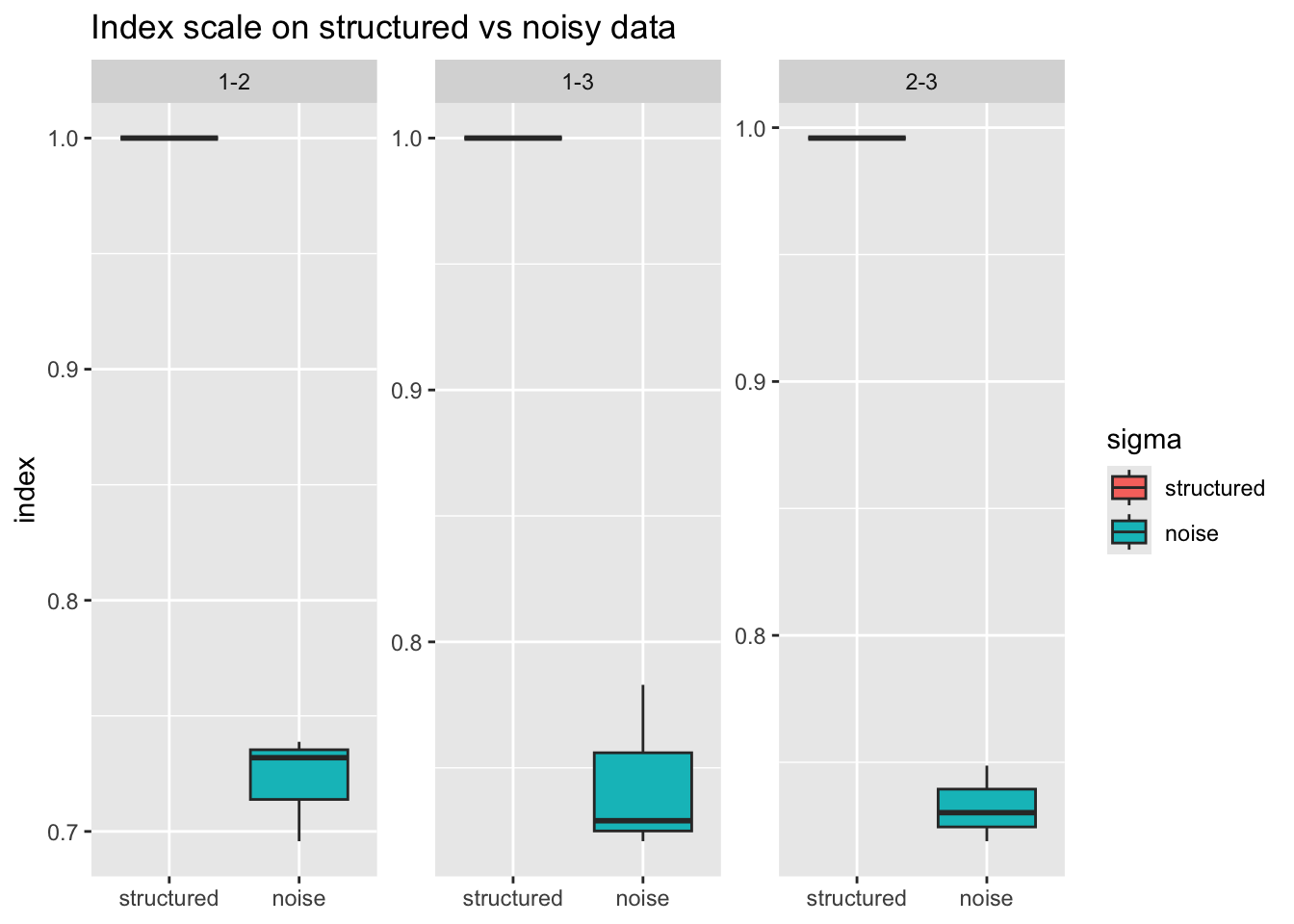
#> 6          1 2     3     2-3          1 0.719

Here sigma = 0 is structured and sigma = 1 is pure noise.

Boxplots: structured vs noise per variable pair

res %>%
  mutate(sigma = factor(sigma, levels = c(0,1), labels = c("structured","noise"))) %>%
  ggplot(aes(x = sigma, y = index, fill = sigma)) +
  geom_boxplot() +
  facet_wrap(~ var_pair, scales = "free_y") +
  labs(
    title = "Index scale on structured vs noisy data",
    x = NULL, y = "index"
  )

Return value

ppi_scale() returns a tibble with columns:

simulation: simulation index
var_i, var_j: the two variable names
var_pair: "var_i-var_j" compact label.
sigma: 0 = structured, 1 = noise
1. Structured value (sigma = 0); compute the index on the actual pair.
2. Noise value (sigma = 1); generate n_obs standard-normal x, y, scale to mean 0 / sd 1, compute the index.
index: the index value from index_fun.

4) Estimating a Noise Threshold for Projection–Pursuit Indices

ppi_noise_threshold() estimates the 95th percentile of a projection pursuit index (PPI) under synthetic noise. This gives you a null threshold: if an observed index on real data exceeds this value, it may indicate non-random structure.

The function supports different noise types via noise_gen() (e.g., Gaussian, $t$ -distributed, Cauchy, microstructure) and lets you set the number of simulations and sample size per simulation.

Function usage

ppi_noise_threshold(
  index_fun,
  n_sim = 100,
  n_obs = 500,
  noise_type  = "gaussian",
  noise_level = 0.01,
  seed = NULL
)

Inputs :

index_fun: a function that returns a single numeric value.
n_sim: number of simulations.
n_obs: sample size per simulation.
noise_type / noise_level: passed through to noise_gen() to control the distribution and its scale.
seed: for reproducibility.

Example Usage

thr <- ppi_noise_threshold(
  index_fun   = scagIndex("stringy"),
  noise_type  = "cauchy",
  noise_level = 0.1,
  n_sim       = 10,
  n_obs       = 100
)
thr
#>       95% 
#> 0.7865055

Return value

ppi_noise_threshold() returns a single numeric: estimated 95th percentile of the index under the specified noise model.

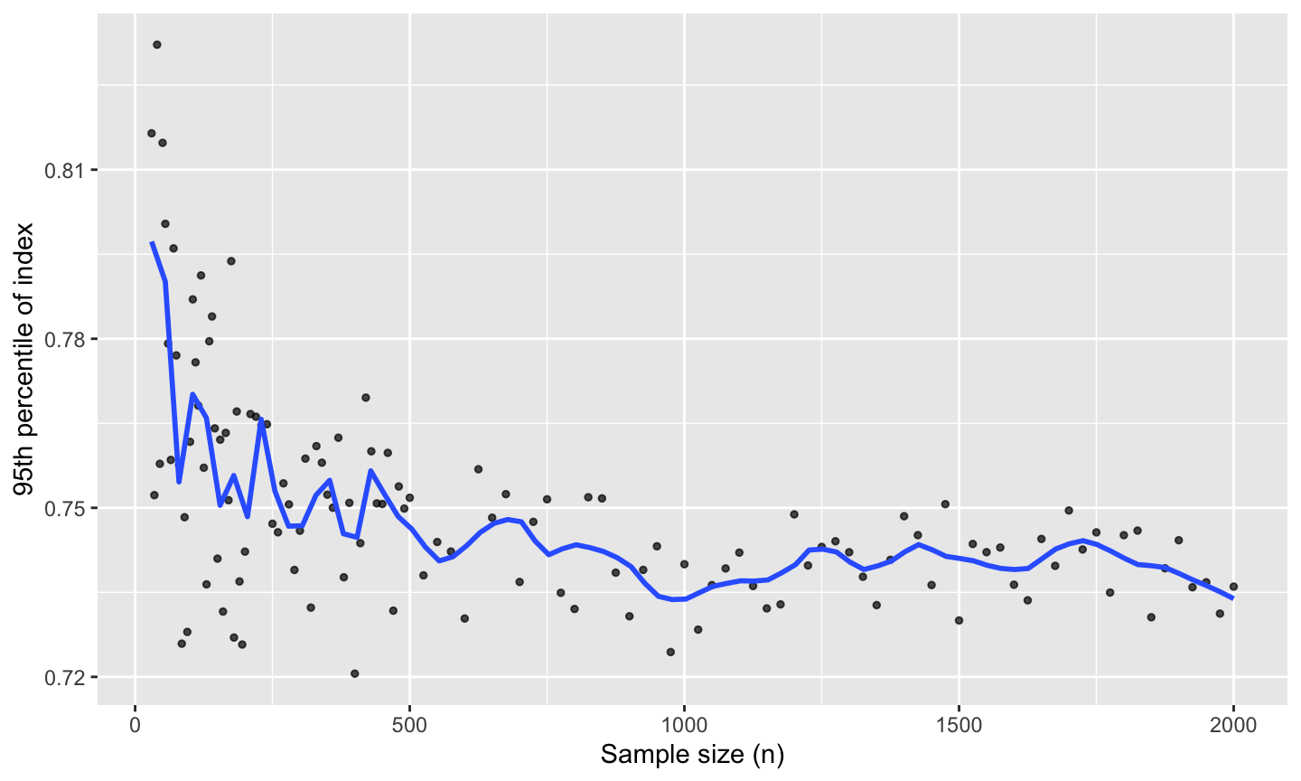
5) Sample-Size Effects for Projection Pursuit Indexes under Gaussian Noise

This demonstrates how to use the ppi_samplesize_effect() function to study how projection pursuit index (PPI) values behave under increasing sample sizes in purely noisy (Gaussian) data. For each size, it computes a specified index function over the samples and records the 95th percentile of index values observed. This helps estimate the distributional behavior of the index under pure noise, depending on sample size. These curves are useful as a null reference: above-curve values may indicate non-random structure.

Function Usage

ppi_samplesize_effect(index_fun, n_sim = 100)

index_fun: a function that accepts the data for one simulation and returns a single numeric index value.
n_sim: the number of simulations per sample size (default 100).

Internally, the function evaluates a grid of sample sizes from 30 up to 2000 (denser at small sizes), simulates n_sim draws for each, and returns the 95th percentile of the resulting index values.

Example Usage

Let’s evaluate the stringy index from the cassowaryr package to see how its values change under noise as the sample size increases.

result <- ppi_samplesize_effect(scagIndex("stringy"), n_sim = 4)
head(result)
#> # A tibble: 6 × 2
#>   SampleSize Percentile95
#>        <dbl>        <dbl>
#> 1         30        0.816
#> 2         35        0.752
#> 3         40        0.832
#> 4         45        0.758
#> 5         50        0.815
#> 6         55        0.800
tail(result)
#> # A tibble: 6 × 2
#>   SampleSize Percentile95
#>        <dbl>        <dbl>
#> 1       1875        0.739
#> 2       1900        0.744
#> 3       1925        0.736
#> 4       1950        0.737
#> 5       1975        0.731
#> 6       2000        0.736

Plot the 95th-percentile

ggplot(result, aes(SampleSize, Percentile95)) +
  geom_point(alpha = 0.7, size = 1) +
  geom_smooth(se = FALSE, method = "loess", formula = y ~ x, span = 0.1) +
  labs(
    x = "Sample size (n)",
    y = "95th percentile of index"
  )

Return value

ppi_samplesize_effect() returns a tibble:

SampleSize: the sample size for that block of simulations
Percentile95: the empirical 95th percentile of the index across the n_sim simulations at that size.

Overview

Packages

1) Generating Synthetic Structures and Noise

Function usage

Example usage

Preview all structures

Polynomial features (type = "polynomial")

noise_gen(): noise distributions

Combining structure + noise

Return value

2) Finding Projection Pursuit Index Mean

Function usage

Example Usage

Return value

3) Comparing Index Scale on Structured vs. Noisy Data

Function Usage

Example usage

Boxplots: structured vs noise per variable pair

Return value

4) Estimating a Noise Threshold for Projection–Pursuit Indices

Function usage

Example Usage

Return value

5) Sample-Size Effects for Projection Pursuit Indexes under Gaussian Noise

Function Usage

Example Usage

Plot the 95th-percentile

Return value

Polynomial features (`type = "polynomial"`)

`noise_gen()`: noise distributions